CellCognition Explorer - User Manual

Create a new data file

Menu: File->New data file
Press the "New File" button in the tool bar

See section Preprocess Raw Image for details.

Open a data file

There are three ways to open a data file:

Menu: File->Open
Click the "Open File" buttonin the tool bar
Drag & Drop: drag a data file from the file manager and drop the file in the main window (anywhere, except in the central gallery viewer)

Batch loading

To keep the application working smoothly on larger data sets, it is possible to load the data in batches. To switch between single batches use the drop down menu Batch No. There is also a Reload button to update the gallery. The default batch size is 10000. It can be changed in the preferences dialog Preferences Dialog.

Sorting

Sorting occurs linearly from the upper left to the bottom right corner. It is necessary to define, dependent on the sort algorithm, at least one reference example. After sorting the reference example will be positioned always in the upper left corner of the view. CellCognition Explorer uses by default the cosine similarity as measure. Other sort algorithms are explained here.

Sorting is controlled most easily by the Sorting Toolbar. It has buttons to sort ascending, descending and a drop down menu to select the sort algorithm.

The Quick Sort-button is used as follows:
First click the button and then a reference example in the gallery. Note the button stays pressed until the procedure has finished. Also the cursor changes to a cross if hovered over the gallery.

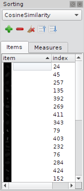
Sorting Dock

The Sorting dock widget allows to define not only, but many cells as reference examples. In this case the arithmetic mean is used as reference example, and the items in the gallery view are ranked by the current sort algorithm.

From top to bottom: Drop down menu for sort algorithm, tool bar with buttons, list view with reference examples. Note: double-click on a item in the list view selects the item in the gallery view to.


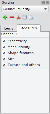
To add/remove items to the sorting dock , simply select/mark one or several items in the graphics view simply press the corresponding button (/)in the dock widget.	The tab "Measurements" allows to sort the objects taking only certain feature groups into account. It is same functionality that is descripted in section Feature Groups, but here, the feature selection applies only for sorting.

Buttons in the tool bar:

Add items

Remove items

Clear items

Sort ascending

Sort descending

Sort algorithms and similarity measures:

Currently four methods/algorithms are available:

Euclidean distance Rank items simply by its euclidean distance to the reference example, works well in low dimensional space.

Cosine Similarity Measures orientation in the feature space not the distance. This is the default sorting method. Robust against outliers in one dimension, works well in high dimensional space.

Class labels First sorts items by class labels, second whether it is a training example, and third by prediction probability. Sorting by class labels

Treatment If during image preprocessing the option DirectoryPerTreatment was used, it is possible to sort the gallery alpha-numerically by treatment, experimental condition resp. If available, class prediction probabilities are used to rank the thumbnails within the treatment groups.

Meaning of class label indicators:

A white (neutral) square indicates that the item, cell resp. is not classified yet.

A colored solid square indicates the class color i.e. the predicted class.

A patterned square with a half circle on top indicates the predicted and annotated class. Color of the square indicates the prediction and the color of the half circle the annotation. Prediction and annotation are not necessarily the same.

Gallery/Thumbnail Viewer

Select items

Double Click to select an item. To select multiple items, click on many items while holding down the Ctrl-button. Drag the mouse while holding down the Ctrl-button will also select multiple items.

Cell Id (tooltip)

If a thumbnail is hoverd by the mouse coursor, a tooltip pops up that shows an Id number (e.g. Id: #99). The same Id number is saved in the first column in the exported csv file.

Multiple color channels

Depending on the input data, CellCognition Explorer displays one or more color channels. It is important to know that CellCognition Explorer does not support RGB images (3-channels, 8bit only). It supports as many color channels as there are in the data. The color display also depends on the input data. The displayed colors are saved to hdf5 along with the numerical image data.
To support multiple colors particularly means that feature vectors calculated from different channels are always concatenated.

View tool bar

Zoom: It is possible to zoom either using the drop down menu or one presses the Shift-key and scroll the mouse wheel.
Classification: Toggle class indicator squares in the left bottom corner of a thumbnail.
Mask: Toggle black background mask of a thumbnail.
Outline: Toggle outlines in a thumbnail.
Treatment: Toggle text that indicates the experimental condition.

view options comparison — View options in comparision.

Contrast Enhancement

Microscope images can be extremely dim and at least for display purpose it is necessary to adjust the contrast parameters i.e. min. and max. value, brightness and contrast. A dock widget supplies this functionality for each channel independently. It can be toggled using the Menu View->Contrast or using the shortcut Alt-Shift-C.

Single channels can be toggled using the checkbox.
The color of single channels can be changed using the corresponding color button.
Select the channel in the drop down menu.
Move the slider to a new value (a tool tip will show the current values of all settings).
For performance reasons the thumbnails are updated if a slider is released.

Classifier training

CellCognition Explorer uses a Support Vector Classifier for multiclass problems (defaut). Other classifiers are One Class Support Vector Machine for outlier detection and a The Manual Classifier is usefull for cases where the sample size is small that no automated classification procedure can be applied.

Similar to the contrast enhancement, there is a dock widget for class training. At the top there is a drop-down menu to select the the classifier and depending on the classifier one can find a Predict-button. The tree view below depends also on the type of the classifier.

Predict

For prediction it is useful to toggle the class label indicators in the gallery viewer i.e. enable the check box Classification in the view tool bar. Then simply press the Predict button and the view gets updated automatically. Sometimes an item can't be predicted because it's feature vector contains NAN's making prediction impossible. The Predict button is color encoded meaning it's indicating a necessary update:

Predict Update required: either the parameters of the classifier or the training set has changed.

Predict No update required.

Function of the buttons:

Add Class Add class to tree view.

Remove Class Remove class from tree view.

Cross Validation & Grid Search Open dialog for cross validation & grid search.

allow reassign If this option is disabled (default) it is not possible to annotate a cell that is already annotated to a different class. This option helps to prevent annotation errors. For reannotation, in case of already wrong annotated cells, enable this option and reannotation is possible without any warning.

Remove Items Remove selected items from annotations.

Clear Treeview Clear class definition and remove all items.

Save Classifier Saves the current classifier.

Load Annotations Load a previously trained classifier.

Save and load a classifier

The Dialogs for saving and loading a classifier are similar. To save a classifier a classifier name and an optional description. It is possible to overwrite a classifier. To load a classifier, a drop down menu shows a list of classifiers saved in the currently opened data file.

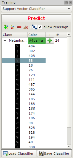
Support vector classifier

Main Elements are a tool bar and annotation tree view:

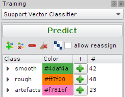
Each class is represented by a line in the tree view. It has a name and color. Name and color can be changed by clicking on the corresponding field in the line. To add items to a particular class, select the items in the the gallery and click on the Add button ( Add button )

Cross validation

Open the dialog by clicking on the symbol . If possible grid search is triggered directly after the dialog pops up. The dialog consists of three tabs and some buttons at the bottom.

Cross Validation Triggers Cross Validation for the current setup of parameters (no grid search).

Grid search Trigger Grid Search.

Apply Apply current parameters to the classifier, leave the dialog open.

Ok Apply current parameters to the classifier and close the dialog.

The first tab (Cross Validation & Grid Search) is to setup parameters manually: five or ten-fold cross validation, grid size for grid search or setup Gamma and C the cost parameter.
The output contains different measures of accuracy: Accuracy, F1,Precession and Recall. A detailed description of the measures can be found in the documentation of the sklearn python package.

Grid search

The result of a grid search is displayed as a contour plot in a logarithmic scale. The yellow cross hairs indicates the optimal parameters. The value displayed is the Accuracy measure mentioned above.

Confusion matrix

The third tab shows the confusion matrix

Matplotlib Navigation Toolbar

By clicking in the plot and using the shortcut t the matplotlib navigationtool shows up at the bottom of a plot. See shortcuts for a detailed description.

Manual Classifier

This classifier convers data sets which small sample numbers. Training a automated classifier is here not possible anymore but one wants to maintain the data output in the same format for subsequent data analysis.
The destinction of training set and test set does not exist. Adding samples to a class in the sidebar, a sample is immediately classified.

Outlier & Novelty Detection

In order to avoid bias due to annotation erros caused by the user, CellCognition Explorer proviedes three different methods for Outlier & Novelty detection.

One Class Support Vector Machine
Kernel Density Estimation
Mahalanobis Distance

Training

Training is performed by adding inliers/ normal objects from one treatment group (e.g. negative control).

Predcition

Prediction performed by density estimation of data points in feature space. Discrimination of normal/abnormal objects depends on the algorithm. For Kernel Density Estimation and Mahalanobis distance a density threshold is estimated by excluding upper the quantile parameter. It excludes the e.g. upper 15 percent of the training set and calculates an ISO curve for density values higher than this threshold. The measure for an object of being an outlier is the euclidean distance between the the ISO curve and the data point in feature space.

The One Class Support Vector Machine calculates the separating hyperplane directly (which is not an ISO curve in that case). Two parametersm, namely Nu and Gamma need to be optimized. The measure for an object of being an outlier is again the euclidean distance between the hyperplane and the data point in feature space.

One Class Support Vector Machine

The parameter setup is slightly different from SVC, since cross validation is not possible one has to setup the parameter semi-automatically.

Nu Minimum fraction of outliers in the training set (training error). In this use case it is a valid assumption to have a very low number of training errors (1%).

Gamma Kernel band width: A smaller value means a lower fraction of support vectors, a higher value means more support vectors. To many support vectors can lead to over fitting.

estimate gamma Estimate Gamma under the constraint that max. 20% of the training samples are support vectors. The value of 20% can be adjusted in the "Preferences" dialog of the application. Nu still has to be set manually.

add item Add items to the training set (annotate items as inlier).

Remove selected items from classifier.

Clear all items from the classifier.

Kernel Density Estimation

Quantile Cutoff used to estimate the denstiy threshold.

Bandwidth Kernel band width.

Estimate Bandwidth Estimate Kernel bandwidth

add item Add items to the training set (annotate items as inlier).

Remove selected items from classifier.

Clear all items from the classifier.

Mahalanobis Distance

Quantile Cutoff used to estimate the denstiy threshold.

add item Add items to the training set (annotate items as inlier).

Remove selected items from classifier.

Clear all items from the classifier.

Image Preprocessing

CellCognition Explorer is an interactive application. To improve performance and prevent unnecessary computation of data some steps in the pipeline are preprocessed such as segmentation, calculation of bounding boxes, features or thumbnails. Image preprocessing is the first step for image analysis and classifier training.

Open Dialog "New File" in the menu "File -> New File":
Click the check boxes to show Outlines and Gallery BBoxes

Image formats:

Currently CellCognition Explorer supports 4D Zeiss LSM images and 4D tiff images (ImageJ version of tiff). 4D means (XYZC) i.e. z-stacks and multiple color channels are supported. In terms of an tiff image one color channel has to be saved as single grey level image. i.e. a multi-color image is a multi-page tiff. CellCognition Explorer does not support RGB images!

Image dimensions:

The tif-standard does not support multidimensional image data as it is used here. Microscope manufacturers and image processing software projects (e.g. ImageJ) came up with their own variant of the format which usually does not comply the tif-standard.
CellCognition Explorer supports reading of lsm files and multipage tifs.
If another format such as PNG are is used to store the data, the dimensional information has to be stored in the file name. In this case open the Image Dimensions dialog by clicking on the button, which opens the Image Dimensions dialog. One can use regular expression to map the images to a 4d stack.

Image Dimensions (multipage tif)

The program uses tifffile to read multipage tiffs.

Dimensions from Regular Expressions

A common case is to save single 2d images and encode the coordinates e.g. color or z-slice into the file name. The program uses a regular expression to read out the 4D coordinate.

Separator	String between single coordinates (e.g. "_")
Z-stack	String at the beginning of the regex group indicating the z-slice.
Channel	String at the beginning of the regex group indicating the color channel.

Example using the settings above:
The file tubulin_P0037_T00001_Crfp_Z1_S1.tif has a single underscore as separator, the z-slice is "1" and the color channel is "rfp".

Treatment and Experimental conditions

By default CellCognition Explorer expects all raw images saved in one single directory, the Image Directory. No information about the experimental conditions is provided. To provide information about the experimental conditions move all images recorded with the same experimental condition to a subdirectory, where the name corresponds to the treatment.
There is a drop down menu in the upper right corner of the Preprocessing Dialog (see figure above) to choose between these two options.

FlatDirectory FlatDirectory Scan the Image directory for lsm and tiff files. No subdirectories are scanned.

DirectoryPerTreatment Scan each subdirectory of the Image directory for lsm and tiff files. No furhter (sub-)subdirectories are scanned. The names of the subdirectories are used as identifiers of the treatment.

Working with multiple colors.

Enabling/disabling channels

The color channels can be toggled by clicking on the corresponding check boxes. The the color map can be changed to. Contrast sliders work similar as those for the gallery viewer. Additionally there is a "Auto"-button that cuts off 1% of the image histogram and the buttons "Min/Max" and "Reset" are self explanatory.

Hint:
It is good practice to use size and intensity filters to reduce the number of foreground objects. Small objects (<100 px�) can be removed since the origin usually from noise and dim objects caused by out-of-focus cells. They have ragged outlines and lot of features evaluate to NAN which make objects unpredictable.

Close Close the dialog.

Start Start image preprocessing for all images.

Segmentation

Segmentation is performed on single color channels. For each channel gets a particular algorithm (plugin) assigned. The program distinguishes between primary- and and non-primary plugins.

Available primary plugins are:

Adaptive Threshold
HoneyComb

Available non-primary plugins are:

Expand
Ring
Shrink
Voronoi

It is possible to assign only one primary plugin a channel. The other channel are segmented either by a non-primary channel or disabled.
It is possible to enable/disable the use of primary plugins in the Preferences dialog.

There are two columns: Channels, Segmentation and there is one row for each color channel. The first row is always for the primary segmentation. e.g. in the screenshot below AdaptiveThreshold will be applied on Channel 1

Channels - common settings for primary segmentation

"Channels 1" Select the color channel in the drop down menu. The list in the menu is updated automatically, if the image directory is changed.

Gallery size Size of the thumbnails (bounding boxes) around foreground objects. This value is fixed after preprocessing is finished and can't be changed later on.

Z Project Standard method for z slice selection. (select, minimum projection, mean, maximum projection max. total intesity)

Outline smoothing Smoothes outlines of foreground objects using a morphological closing operation followed by an morphological opening. Dim out of focus cells have usually a ragged outline causing a lot of features to be invalid i.e. their value is NaN. Smoothing outlines helps to overcome this problem and increases classifier performance. The parameter is the size of the structuring element of the morphological operation. Negative values disable outline smoothing.

Adaptive Threshold

Min. contrast Minimum contrast (i.e. threshold) for local adaptive threshold segmentation.

Mean radius Radius in pixels for the Gaussian blurring filter.

Window size Filter size used for local adaptive thresholding.

Watershed Enable/disable watershed segmentation.

Seeding size Size parameter for finding seed for the watershed segmentation. Seeding is applying minimum and maximum filters. This parameter is the the size of the filters. There is only one seed within an area of radius seeding size.

Object Filters

Intensity filter Remove objects outside the intensity range (min, max). A value of -1disables the border e.g. (10, -1) filters all objects with a mean intensity lower than 10 (uint8 gray values).

Size filter Remove foreground objects outside the range (min, max). A value of -1 disables the border e.g. (100, -1) filters all objects smaller than 100 px�.

Remove border objects Removes all foreground objects that touches the image boundary (border objects are artefacts).

Fill holes Topologically close all foreground objects.

Intensity normalization Renormalize input images from min/max (by default 0, 255) to unsigned 8 bit images. The data type of the images determines the range of the values. By default the values 0 and 255 (8bit images) are used. For 16bit and higher bit depths minimum and maximum values of the current image are proposed.

Non-Primary Segmentation Plugins

Drop down menu One of Expand, Shrink, Ring or Voronoi
Dist inner Distance between primary outline and shrunk outline (any value from 0 to inf)
Dist outer Distance between primary outline and expanded outline (any value from 0 to inf)

Intensity Normalization Renormalize input images from min/max (by default 0, 255) to unsigned 8 bit images. The data type of the images determines the range of the values. By default the values 0 and 255 (8bit images) are used. For 16bit and higher bit depths minimum and maximum values of the current image are proposed.

Load/Save segmentation settings

Segmentation settings are automatically saved to the data file. Additionally it is possible to save settings as xml file which can be edited manually. Loading or reusing of settings is therefore possible either from the data file or from xml.

Preferences

Application Preferences can be found in the Menu File -> Preferences.

Preferences - General

Use complementary colors for outlines If enabled, outlines are displayed in complementary colors e.g. thumbnails are red, outlines are cyan. For gray level images the outlines are yellow. If this option is disabled outlines use the same color as the thumbnails.

Default similarity metric Set the default metric for the method Quick Sort

Feature Grouping Default feature grouping used in the feature selection dialog.

Enable Segmentation Plugins If enabled, the drop down menu in the in the segmentation dialog is shown allow different primary segmentation plugins. By default the plugin AdaptiveThreshold is used.

Max. fraction of outliers Parameter estimation for the One Class SVM assumes a that max. 20% of the trainings samples are support vectors. This option allows to change the value. A high fraction of support vectors may lead to overfitting.

Preferences - Data IO

Hdf5 compression Use "gzip", "lzf" or "None" as compression algorithm. Degree of compression ranges from 1 (low compression) to 9 (high compression). "lzf" has no options. Default is gzip, 4. This is a good compromise of speed vs. compression factor. It is recommended to not change the default.

Batch Size Default batch size to keep the application working smoothly. The Batch size determines the max. number of thumbnails that are shown in the gallery view. See the Batch Toolbar how to control the Batch loading feature.

Data Export If on save raw image data to hdf5. Default is off.

Preferences - Features

Hidden in the preferences dialog are the setting for the compuational feature groups. CellCognition Explorer uses the the cellcognition framework for feature calculation. A compuational feature group defines one block of features that is calculatated together in a computational effective manner. For instance Haralick features: the coocurrence matrix is only calculated once since all Haralick features with the same distance parameter use the same matrix.
A detailed description of the cellcognition feature groups can be found at doc.cellcognition.org.

Note:
The settings for the computational feature groups apply to all color channels. It is recommended to turn all by default on, except the Spot Features which can be used to descripe bright speckles inside a foreground object.

Data file formats:

The term "data file" which was used quite often above means either a hdf5 file, or a cellh5 file.

Hdf5 - CellCognition Explorer saves its data to hdf5 which is optimized structures for fast IO. This supports the paradigm of interactivity of the application. All data and settings which where used to produce the data sets and classifiers go into this file.
CellH5 - It is also possible to load data from cellh5 files and save classifier data to a cellh5 file. Cellh5 data structures are not as performant, but store much larger data sets, and support data from screening plates (plate layout). Further cellh5 supports saving of tracking and event data. The cellh5 navigation tool bar enables navigation and loading from different plates, wells and sites. Future version will also enable loading of event data, loading of multiple color channels and train merged channel classifiers.

Data export

It is possible to export data for further analysis with external programs. The export format is a simple csv-file since any data analysis program can import csv files.

See the menu Data to proceed

Save View Panel as image Saves the current gallery view as png image (large images size!).

Save counting statistics For a quick overview over the counts per class and treatment after classification. Here is an example. The counting statistics does not take samples from the training set i.e. samples used to train the classifier, into account.

Save data to csv Saves data of all cells in the gallery view in a csv file. The convetion is one line per cell. Each column represents a different attribute. i.e. id, class name, class label, treatment, training sample, feature(s). Here is an example. The meaning of the features is documented somewhere else.
Note: The first column is the cell Id number. It establishes a relation between destinct thumbmail (Id appears it the tooltip) and a line in the exported table.

Feature groups

The current implementation uses the descriptors set of the cellcognition-framework. It consists of 239 single values including simple features like mean intensity or roisize but also more abstract ones like Haralick features, descriping the texture of an object. It is important to note that different color channels are treated independently i.e. it is possible to toggle features (or feature groups) always separately.
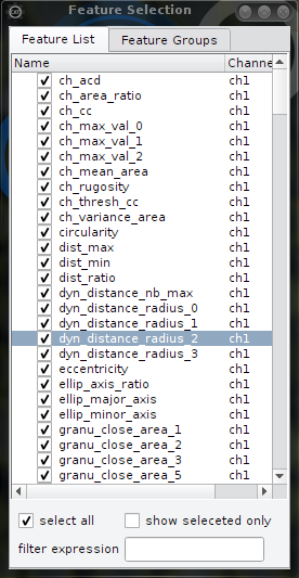
By Default all 239 features are used for analysis but it is possible to select only a subset and there are two ways to do this. Select feature by name and select feature by group. First open the Feature selection Dialog (Menu: View):

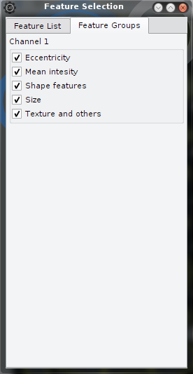
Select features by name	Select features by group
This is the general case. Only selected (checked) features are used for sorting and classification.	Here it is possible to toggle features in groups. Feature groups are provided alongside with the feature names by the hdf5 and cellh5 files and updated automatically if a file is opened. Feature groups provide a more intutitive access to the choise of the features since feature names are choosen usually cryptically. Be aware that feature groups are arbitrary.

Both feature names and feature groups are saved in the hdf file (or ch5 file resp.) and both depend on the image processing applicaton that processed the input data. CellCognition Explorer and Cellcognition use the same feature set.

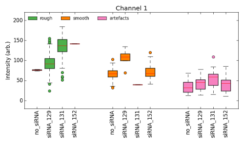
Statistical Plots:

Simple box- and bar graphs can be displayed using either the corresponding menu or shortcut. The plots give a quick overview over the class counts and dedicated features. Each color channel generates an independent plot. The colors of the bars are defined by the user in the class definition.

Please note that the plots adjust the ranges and scales automatically. Custom adjustment is possible using the toolbar at the bottom of each plot.

Following plots are available:

Bargraph grouped by class.
Bargraph grouped by treatment.
Boxplot - Intesity
Boxplot - Size
Boxplot - Standard Deviation of Intesity

	Add items
	Remove items
	Clear items
	Sort ascending
	Sort descending

Euclidean distance	Rank items simply by its euclidean distance to the reference example, works well in low dimensional space.
Cosine Similarity	Measures orientation in the feature space not the distance. This is the default sorting method. Robust against outliers in one dimension, works well in high dimensional space.
Class labels	First sorts items by class labels, second whether it is a training example, and third by prediction probability.
Treatment	If during image preprocessing the option DirectoryPerTreatment was used, it is possible to sort the gallery alpha-numerically by treatment, experimental condition resp. If available, class prediction probabilities are used to rank the thumbnails within the treatment groups.

	A white (neutral) square indicates that the item, cell resp. is not classified yet.
	A colored solid square indicates the class color i.e. the predicted class.
	A patterned square with a half circle on top indicates the predicted and annotated class. Color of the square indicates the prediction and the color of the half circle the annotation. Prediction and annotation are not necessarily the same.

Predict	Update required: either the parameters of the classifier or the training set has changed.
Predict	No update required.

	Add class to tree view.
	Remove class from tree view.
	Open dialog for cross validation & grid search.
allow reassign	If this option is disabled (default) it is not possible to annotate a cell that is already annotated to a different class. This option helps to prevent annotation errors. For reannotation, in case of already wrong annotated cells, enable this option and reannotation is possible without any warning.
	Remove selected items from annotations.
	Clear class definition and remove all items.
	Saves the current classifier.
	Load a previously trained classifier.

Cross Validation	Triggers Cross Validation for the current setup of parameters (no grid search).
Grid search	Trigger Grid Search.
Apply	Apply current parameters to the classifier, leave the dialog open.
Ok	Apply current parameters to the classifier and close the dialog.

Nu	Minimum fraction of outliers in the training set (training error). In this use case it is a valid assumption to have a very low number of training errors (1%).
Gamma	Kernel band width: A smaller value means a lower fraction of support vectors, a higher value means more support vectors. To many support vectors can lead to over fitting.
	Estimate Gamma under the constraint that max. 20% of the training samples are support vectors. The value of 20% can be adjusted in the "Preferences" dialog of the application. Nu still has to be set manually.
	Add items to the training set (annotate items as inlier).
	Remove selected items from classifier.
	Clear all items from the classifier.

Quantile	Cutoff used to estimate the denstiy threshold.
Bandwidth	Kernel band width.
	Estimate Kernel bandwidth
	Add items to the training set (annotate items as inlier).
	Remove selected items from classifier.
	Clear all items from the classifier.

	FlatDirectory	Scan the Image directory for lsm and tiff files. No subdirectories are scanned.
	DirectoryPerTreatment	Scan each subdirectory of the Image directory for lsm and tiff files. No furhter (sub-)subdirectories are scanned. The names of the subdirectories are used as identifiers of the treatment.

Close	Close the dialog.
Start	Start image preprocessing for all images.

"Channels 1"	Select the color channel in the drop down menu. The list in the menu is updated automatically, if the image directory is changed.
Gallery size	Size of the thumbnails (bounding boxes) around foreground objects. This value is fixed after preprocessing is finished and can't be changed later on.
Z Project	Standard method for z slice selection. (select, minimum projection, mean, maximum projection max. total intesity)
Outline smoothing	Smoothes outlines of foreground objects using a morphological closing operation followed by an morphological opening. Dim out of focus cells have usually a ragged outline causing a lot of features to be invalid i.e. their value is NaN. Smoothing outlines helps to overcome this problem and increases classifier performance. The parameter is the size of the structuring element of the morphological operation. Negative values disable outline smoothing.

Min. contrast	Minimum contrast (i.e. threshold) for local adaptive threshold segmentation.
Mean radius	Radius in pixels for the Gaussian blurring filter.
Window size	Filter size used for local adaptive thresholding.
Watershed	Enable/disable watershed segmentation.
Seeding size	Size parameter for finding seed for the watershed segmentation. Seeding is applying minimum and maximum filters. This parameter is the the size of the filters. There is only one seed within an area of radius seeding size.

Intensity filter	Remove objects outside the intensity range (min, max). A value of -1disables the border e.g. (10, -1) filters all objects with a mean intensity lower than 10 (uint8 gray values).
Size filter	Remove foreground objects outside the range (min, max). A value of -1 disables the border e.g. (100, -1) filters all objects smaller than 100 px�.
Remove border objects	Removes all foreground objects that touches the image boundary (border objects are artefacts).
Fill holes	Topologically close all foreground objects.
Intensity normalization	Renormalize input images from min/max (by default 0, 255) to unsigned 8 bit images. The data type of the images determines the range of the values. By default the values 0 and 255 (8bit images) are used. For 16bit and higher bit depths minimum and maximum values of the current image are proposed.

Drop down menu	One of Expand, Shrink, Ring or Voronoi
Dist inner	Distance between primary outline and shrunk outline (any value from 0 to inf)
Dist outer	Distance between primary outline and expanded outline (any value from 0 to inf)
Intensity Normalization	Renormalize input images from min/max (by default 0, 255) to unsigned 8 bit images. The data type of the images determines the range of the values. By default the values 0 and 255 (8bit images) are used. For 16bit and higher bit depths minimum and maximum values of the current image are proposed.

Use complementary colors for outlines	If enabled, outlines are displayed in complementary colors e.g. thumbnails are red, outlines are cyan. For gray level images the outlines are yellow. If this option is disabled outlines use the same color as the thumbnails.
Default similarity metric	Set the default metric for the method Quick Sort
Feature Grouping	Default feature grouping used in the feature selection dialog.
Enable Segmentation Plugins	If enabled, the drop down menu in the in the segmentation dialog is shown allow different primary segmentation plugins. By default the plugin AdaptiveThreshold is used.
Max. fraction of outliers	Parameter estimation for the One Class SVM assumes a that max. 20% of the trainings samples are support vectors. This option allows to change the value. A high fraction of support vectors may lead to overfitting.

Hdf5 compression	Use "gzip", "lzf" or "None" as compression algorithm. Degree of compression ranges from 1 (low compression) to 9 (high compression). "lzf" has no options. Default is gzip, 4. This is a good compromise of speed vs. compression factor. It is recommended to not change the default.
Batch Size	Default batch size to keep the application working smoothly. The Batch size determines the max. number of thumbnails that are shown in the gallery view. See the Batch Toolbar how to control the Batch loading feature.
Data Export	If on save raw image data to hdf5. Default is off.

Save View Panel as image	Saves the current gallery view as png image (large images size!).
Save counting statistics	For a quick overview over the counts per class and treatment after classification. Here is an example. The counting statistics does not take samples from the training set i.e. samples used to train the classifier, into account.
Save data to csv	Saves data of all cells in the gallery view in a csv file. The convetion is one line per cell. Each column represents a different attribute. i.e. id, class name, class label, treatment, training sample, feature(s). Here is an example. The meaning of the features is documented somewhere else. Note: The first column is the cell Id number. It establishes a relation between destinct thumbmail (Id appears it the tooltip) and a line in the exported table.